Detectors
Detectors are Flat Components, when photons are traced to them, these photons are binned into pixels which can then be viewed. In the future, detectors will be able to simulate noise and interactions such as split events. Then you will be able to use detectors in your Instrument to generate sample data and test your data analysis or event detection beforehand.
Creating a Detector
A Collimator Plate requires the following arguments:
- x,y,z - The spatial coordinates of the center of the plate. See Flat Component
- nx,ny,nz - The components of the normal vector. See Flat Component
- sx,sy,sz - The components of the surface vector. See Flat Component
- q - The quantum efficiency of the detector. This input should be a float that ranges from 0 to 1, it defaults to 1. This quantity specifies the probability that a given photon will be detected if it impacts the Detector.
- l - The length of the Collimator Plate. This is the extent of the Component in the direction of the surface vector
- l must be in units of length. See the section on Astropy Units.
- w - The width of the Collimator Plate. This is the extent of the Component in the direction of the cross product of the surface and normal vectors (sxn).
- w must be in units of length. See the section on Astropy Units.
- xpix - The number of pixels along the width of the axis, i.e: how many pixels lie along a line parallel to the x-unit vector (the surface-cross-normal vector).
- ypix - The number of pixels along the length of the axis, i.e: how many pixels lie along a line parallel to the y-unit vector (the surface vector).
- fieldfree - The depth of the field free region of the detector. Defaults to 15 microns.
- field free must be in units of length, see the section on Astropy Units
- depletion - The depth of the depletion region of the detector. This parameter currently does not have any effect on the Detector. Defaults to 3 microns.
- depletion must be in units of length, see the section on Astropy Units
- considersplits - A boolean to determine if split events should be considered. Should be True if you want to simulate split events, note that this will slow down the view() function significantly. Defaults to False.
- steps - If considersplits is True, the split events will be calculated using this number of steps. A lower number of steps will be less accurate but will run faster. For small splits (taking up only a few pixels), fewer steps is acceptable.
Warning
Unlike other Flat Components, Detectors MUST have a length and width defined. If no arguments are passed, these dimensions will both default to 1 mm.
Moving a Detector
Detector objects inherit translate, rotate, and unitrotate from Flat Component, see the function usage here
Trace
Trace is a function of all descendents of Flat Component. When called, rays will be traced to the surface and any photons which fall outside of the detector’s range will be removed. If placed in an Instrument object and simulated, trace will be called automatically.
Trace takes the following inputs:
- rays - The Rays object which you want to trace to the Detector.
- considerweights - This is a boolean which should be true if your photons are weighted. If True, it will be the photon’s weights which are affected by the Detector’s quantum efficiency, so no photons will be removed from the Rays object. See the section on photon weighting.
- eliminate - This is an argument of every trace function. It is a string which defaults to “remove”. If it is the default value, photons which miss the detector will be removed from the Rays object. If it is anything else, the x-position of the missed photons will be set to NaN. This argument is mostly used by Combination objects.
The Trace function will modify the Rays object in place. It will return a tuple that gives information about how many photons made it to the detector. This tuple is used by Instrument objects to analyze the efficiency of the entire Instrument.
Add Gaussian Noise
The function addGaussianNoise tells the Detector what type of noise should be added to the pixel array.
addGaussianNoise takes the following inputs:
- mean - The mean of the normal distribution being added to the array, defaults to 0.
- std - The standard deviation of the normal distribution being added to the array, defaults to 1.
Note that this function has no immediate impact on the Detector’s pixel array. Calling this function just saves the arguments so that when the view() function is called, it knows what kind of noise to add.
Add Custom Noise
If you have a frame that characterizes the noise of the detector (like a bias frame or dark frame), you can add it in the addNoise() function to generate accurate noise when view() is called.
addNoise() takes the following inputs:
- noise - A 2D array the same size as the pixel array which has the noise value for each pixel.
When view() is called, each pixel will be given a noise value according to a poisson distribution where lambda is given by the noise argument in addNoise.
Note: addNoise() can be called more than once. If this is done, the subsequent noise arrays will be averaged together. This allows you to add in many noise files to get an accurate estimate of the detector’s noise.
Note: if addGaussianNoise() is called after addNoise(), the noise arrays will be lost.
Finally, when view() is called, the most recent noise function called will be used to add noise values.
Example:
from prtp.Rays import Rays
from prtp.Detector import Detector
import numpy as np
import matplotlib.pyplot as plt

r = Rays()

d = Detector(xpix=100,ypix=100)

# Add 5 channels of noise
noise = np.zeros((100,100))
for i in range(5):
   noise[:,20*i:20*(i+1)] += np.random.choice([8,12,16,20])

d.addNoise(noise)

a = d.view(r)

plt.figure()
plt.imshow(a)
plt.show()
View
The function view returns the pixel array. If you wish to have photons on the pixel array, you must specify the Rays object when calling view.
view takes the following arguments:
- rays - The Rays object you want to include on the Detector’s surface. This argument defaults to None, in which case no photons will be included but the array will still be returned.
- The Detector cannot tell if the Rays have been traced to the surface before calling view. If you call view before tracing Rays, you will still see the photons, but they will not be in the correct locations.
Note: Once you have the pixel array, the best way to see it is to use pyplot’s “imshow” function, see examples at the bottom of this page.
Note: If the value for considersplits of this Detector is True, view() will call the split() function. A helper function that will bin the charge cloud from each photon into the adjacent pixels.
Warning
Calling view when the photons have no wavelength will generate an error.
Reset
The function reset takes no arguments and sets all of the pixel values back to 0.
Examples
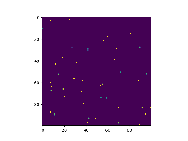
Basic Photon Trace
This example will trace a circular beam of photons to a Detector’s surface and then plot them.
import matplotlib.pyplot as plt
from prtp.Detector import Detector
from prtp.Sources import CircularBeam
import astropy.units as u

s = CircularBeam(num=10000,rad=4*u.mm,wave=100*u.eV)
rays = s.generateRays()

d = Detector(x=0*u.mm,y=0*u.mm,z=2*u.mm,
   nx=0,ny=0,nz=1,sx=0,sy=1,sz=0,q=1.,
   l=10*u.mm,w=10*u.mm,xpix=100,ypix=100)

d.trace(rays)
arr = d.view(rays)

plt.figure()
plt.imshow(arr)
plt.show()
When executed, the code produces the following plot:

As it was defined, this detector has dimensions 10mm x 10mm and has 100 pixels on a side.
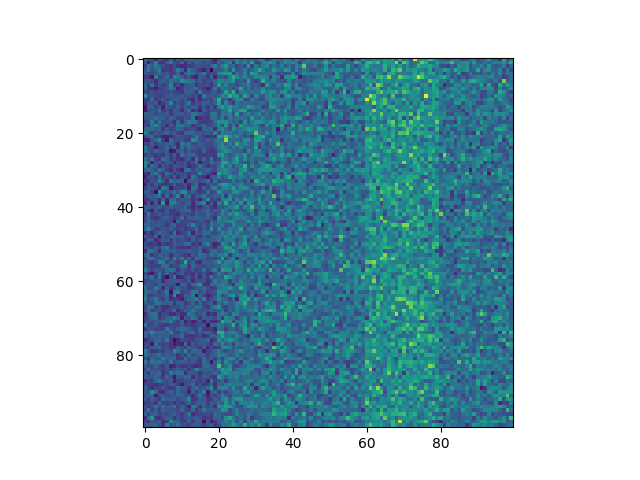
Photon Trace with Noise
This example will perform the same trace as before but with Gaussian noise added beforehand.
import matplotlib.pyplot as plt
from prtp.Detector import Detector
from prtp.Sources import CircularBeam
import astropy.units as u

s = CircularBeam(num=10000,rad=4*u.mm,wave=100*u.eV)
rays = s.generateRays()

d = Detector(x=0*u.mm,y=0*u.mm,z=2*u.mm,
   nx=0,ny=0,nz=1,sx=0,sy=1,sz=0,q=1.,
   l=10*u.mm,w=10*u.mm,xpix=100,ypix=100)

d.trace(rays)
d.addGaussianNoise(mean=20,std=1)
arr = d.view(rays)

plt.figure()
plt.imshow(arr)
plt.show()
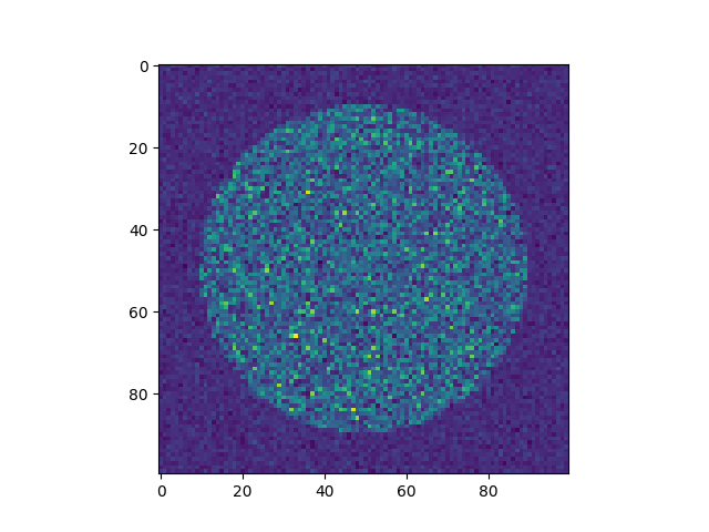
Note that the call to addGaussianNoise() could have been performed before or after the call to trace(), so long as view() was called last.
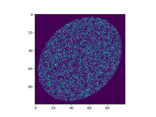
Misaligned Photon Trace
This example will trace photons that do not hit the detector dead on, rather, the detector is at a slight angle with respect to the incoming photons.
import matplotlib.pyplot as plt
from prtp.Detector import Detector
from prtp.Sources import CircularBeam
import astropy.units as u

s = CircularBeam(num=10000,rad=4*u.mm,wave=100*u.eV)
rays = s.generateRays()

d = Detector(x=0*u.mm,y=0*u.mm,z=2*u.mm,
   nx=0,ny=0,nz=1,sx=0,sy=1,sz=0,q=1.,
   l=10*u.mm,w=10*u.mm,xpix=100,ypix=100)

d.rotate(theta=40*u.deg,ux=1,uy=1,uz=0)

d.trace(rays)

arr = d.view(rays)

plt.figure()
plt.imshow(arr)
plt.show()
Split Event
This example will consider split events. It does so by specifying considersplits=True when the Detector is defined.
import matplotlib.pyplot as plt
from prtp.Detector import Detector
from prtp.Sources import CircularBeam
import astropy.units as u

s = CircularBeam(num=100,rad=8*u.mm,wave=100*u.eV)
rays = s.generateRays()

d = Detector(x=0*u.mm,y=0*u.mm,z=2*u.mm,
   nx=0,ny=0,nz=1,sx=0,sy=1,sz=0,q=1.,
   l=10*u.mm,w=10*u.mm,xpix=100,ypix=100,
   considersplits=True,steps=50)

d.trace(rays)
arr = d.view(rays)

plt.figure()
plt.imshow(arr)
plt.show()